Curve Parameterization For Mere Mortals

Introduction

In our previous article, we have seen how to define and use curves to create paths.

A curve is a smooth parametric function defined as:

$C(t) = (x(t), y(t), z(t))$

where $t$ is the parameter, and $x(t), y(t), z(t)$ are functions that define the curve.

Suppose that we want to sample some points from the curve.

Hmm, simple! It suffices to divide the interval $([0,1])$ into n sub-intervals and evaluate at each endpoint.

Example:

float nPoints = 512;

for (int i = 0; i < nPoints; i++) 
{
    float dt = 1.0f / (nPoints - 1.0f);
    float t = i * dt;
    Draw(curve.Get(t));
}

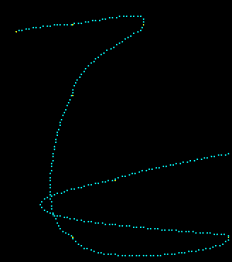
When we draw the sampled points, we obtain a rough approximation of the curve, as in the image below.

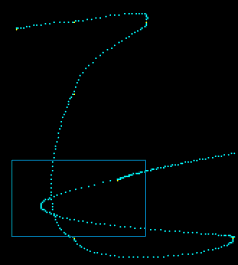
As we can see, the obtained points are unevenly spaced, even if the intervals are evenly spaced. The artifacts can become less visible if we sample more densely. For example, we may choose a value nPoints = 10000.

We can also try to modify the sampling method to obtain an evenly spaced sampling. But before we do that, we need to review some useful concepts.

Differential Geometry of the Curve

If a curve represents the path of a particle, then the velocity of the particle at a given point ( P ) is expressed by a vector, called the tangent vector to the curve. The curve is a function that takes a parameter ( t ) between ( 0 ) and ( 1 ) and returns a 3D vector. If we calculate the derivative of the curve at a particular point, we obtain the velocity ( V ):

$V(t) = \frac{dC}{dt}$

So, we have seen how to calculate the velocity (tangent) of the curve at a particular point. For further details, see the previous post. Now we can build a curve, draw it, and calculate the tangent vector at a point.

Another useful function is the calculation of the length of our curve! Let's devise a simple method for that.

Approximation of the Length

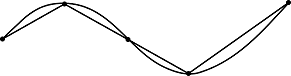
A useful approximation relies on a finite number of points on the curve using line segments to create a polygonal path. The total length of the curve can be found by summing the lengths of each line segment. Another method for finding the length is by integrating the function:

$L = \int_{t_1}^{t_2} \left| V(t) \right| dt$

An intuitive way to look at the formula is to consider the first approach of length approximation. We have seen that we can approximate the total length by summing the lengths of the line segments. We are doing the same here. The length can be considered as an infinitesimal segment, and the integral is just summing all those infinitesimal segments.

To calculate the part of the curve between two points at $( t_1 )$ and $( t_2 )$, it suffices to compute the integral:

Let's translate those formulas into code! We don’t have to explicitly evaluate the integral; we can approximate it numerically. Various techniques exist for numerical integration. We use Simpson’s rule, based on the formula:

$\int_a^b f(x) dx \approx \frac{h}{6} \left[ f(a) + 4f\left(\frac{a+b}{2}\right) + f(b) \right]$

Simpson's Rule Implementation:

float VelocityIntegral(float t1, float t2, int maxIntegrationSteps) 
{
    float from = t1;
    float to = t2;
    float n = maxIntegrationSteps;
    float h = (to - from) / n;
    float sum1 = 0.0f;
    float sum2 = 0.0f;
    int i;

    for (i = 0; i < n; i++) 
    {
        sum1 += GetVelocity(from + h * i + h / 2.0f);
    }

    for (i = 1; i < n; i++) 
    {
        sum2 += GetVelocity(from + h * i);
    }

    return (float)(h / 6.0 * (GetVelocity(from) + GetVelocity(to) + 4.0 * sum1 + 2.0 * sum2));
}

Natural, Arc-Length, or Unit-Speed Parameterization

We have seen that if a curve represents the path of a particle, then the velocity of the particle at a given point ( P ) is expressed by a vector, called the tangent vector to the curve. To obtain the vector, it is sufficient to take the derivative. As we have also remarked in Figure-1, in general, the velocity of the particle is not constant. This can be problematic if we want to use the curve as a path.

So we need to change the velocity of the path traversal. Let $( s(t) )$ be a function such that:

$s(t) = \int_0^t \| V(\tau) \| d\tau$

Let:

$t = s^{-1}(y)$

where $( t(s) )$ is the inverse of $( s(t) )$.

We have:

$\frac{dt}{ds} = \frac{1}{\| V(t) \|}$

This means that the velocity is constant, and thus:

Now we have $( s(t) )$, we need to compute its inverse. So for every value of $( t )$, we find the corresponding value of $( s )$. The closed-form expression of $( s )$ can be very complex. So we once again need numerical approximations.

To find the inverse $( t )$ for a particular value $( y )$:

We now need a method for finding the root of the function $( g(t) = s(t) - y )$.

The bisection method is a root-finding method that repeatedly bisects an interval and then selects a subinterval in which a root must lie. It is a robust method, but it is also relatively slow.

Bisection Method Implementation:

double FindRoot(Func<double, double> function, double a, double b, double tolerance) 
{
    double x = (a + b) / 2.0;

    if (a > b) 
    {
        return x;
    }

    double fa = function(a);
    double fb = function(b);

    if (fa * fb > 0) 
    {
        return x;
    }

    do 
    {
        x = (a + b) / 2.0;
        double f = function(x);

        if (f * fa > 0) 
        {
            a = x;
        }
        else 
        {
            b = x;
        }
    } while (b - a > tolerance);

    return x;
}

Finally, we can find the value of $( t )$. What we do is to choose a value $( y )$, find the corresponding value $( t )$, and then evaluate the curve at $( t )$.

Voilà! 🎉